【医療画像AI】U-Netを使ってX線画像の領域分割やってみた【Python】#006
こんにちは!こーたろーです。
今回はU-Netというモデルを使った領域分割を行ってみます。
画像の中に何があるかを区別するために、画像の対象を区切って利用することがあります。
その時に必要となってくるのが、この領域分割です。
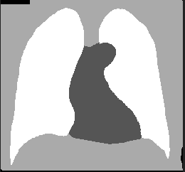
こちらの図のように、身体・肺・心臓・背景のように分割したい場合に、U-Netを使って学習させたモデルがどのぐらい領域分割できるか試してみます。
それでは早速始めていきます。
データの準備
データは毎度おなじみの日本放射線技術学会の画像部会が公開しているデータを使用します。
miniJSRT_database | 日本放射線技術学会 画像部会
リンクをスクロールして、「Segmentation01」をダウンロードして、展開後、ホームディレクトリに設置します。
今回利用しているデータは、分割後の画像はpng、現画像はbmpとなっていることに注意します。
なお、分割後の画像についてですが、画素数は
肺 :255
心臓:85
身体:50
背景:0
となっています。
それでは、データを読み込んでいきたいと思います。
import os
import cv2
import numpy as np
from keras.layers import Input, Conv2D, MaxPooling2D, UpSampling2D, BatchNormalization
from keras.layers.merge import concatenate
from keras.models import Model
import matplotlib.pyplot as plt
まずはライブラリをインポートしておきます。
次に、今回の処理で指定する画像のサイズと学習のエポック数だけ定義しておきます。
IMAGE_SIZE = 64
EPOCHS = 10
データの読み込み
まずは、データの前処理を行っていきます。
続いて、大量のデータが複数のフォルダに分かれていることから、データを読み込むための関数を準備します。
関数では、ホームディレクトリにおいたファイルのパスと、変更後の画像サイズを指定していきます。
def load_images(inputpath, imagesize):
    imglist = []

    for root, dirs, files in os.walk(inputpath):
        files[:] = [file for file in files if not file.startswith(('__', '.'))]

        for fn in sorted(files):
            bn, ext = os.path.splitext(fn)
            filename = os.path.join(root, fn)
            testimage = cv2.imread(filename, cv2.IMREAD_GRAYSCALE)
            height, width = testimage.shape[:2]
            testimage = cv2.resize(testimage, (imagesize, imagesize), interpolation = cv2.INTER_AREA)
            testimage = np.asarray([testimage], dtype=np.float64)
            testimage = np.asarray(testimage, dtype=np.float64).reshape((1, imagesize, imagesize))
            testimage = testimage.transpose(1, 2, 0)

            imglist.append(testimage)
    imgsdata = np.asarray(imglist, dtype=np.float32)

    return imgsdata, sorted(files)
そしてデータを読み込みます。
image_train, image_train_filenames = load_images("./segmentation/org_train/", IMAGE_SIZE)
label_train, label_train_filenames = load_images("./segmentation/label_train/", IMAGE_SIZE)

image_test, image_test_filenames = load_images("./segmentation/org_test/", IMAGE_SIZE)
label_test, label_test_filenames = load_images("./segmentation/label_test/", IMAGE_SIZE)
データの前処理
続いて、データの前処理です。今回、領域は肺とそれ以外を区別するものを作ろうと考えています。
そのため、前処理段階で、画素数が255のものはそのまま残し、それ以外を0にする処理を加えます。
そして、最後に正規化を行います。
for organ in range(0, len(label_train)):
    for i in range(0, IMAGE_SIZE):
        for j in range(0, IMAGE_SIZE):
            if(label_train[organ][i][j][0] != 255):
                label_train[organ][i][j][0] = 0
            else:
                label_train[organ][i][j][0] = 255

for organ in range(0, len(label_test)):
    for i in range(0, IMAGE_SIZE):
        for j in range(0, IMAGE_SIZE):
            if(label_test[organ][i][j][0] != 255):
                label_test[organ][i][j][0] = 0
            else:
                label_test[organ][i][j][0] = 255

image_train /= np.max(image_train)
label_train /= np.max(label_train)
image_test /= np.max(image_test)
label_test /= np.max(label_test)
U-Netのネットワークの定義
U-Netのライブラリ(パッケージ)は一応公開されているようでしたが、今回は手組みしてみました。
ちなみにいろいろな参考文献・書籍などをみながら、次のネットワークが一番わかりやすかったので参考にしてみました。
def network_unet():
    input_data = Input(shape=(IMAGE_SIZE, IMAGE_SIZE, 1))

    encode1 = Conv2D(64, kernel_size=3, strides=1, activation="relu", padding="same")(input_data)
    encode1 = BatchNormalization()(encode1)
    encode1 = Conv2D(64, kernel_size=3, strides=1, activation="relu", padding="same")(encode1)
    encode1 = BatchNormalization()(encode1)
    downsample1 = MaxPooling2D(pool_size=2, strides=2)(encode1)

    encode2 = Conv2D(128, kernel_size=3, strides=1, activation="relu", padding="same")(downsample1)
    encode2 = BatchNormalization()(encode2)
    encode2 = Conv2D(128, kernel_size=3, strides=1, activation="relu", padding="same")(encode2)
    encode2 = BatchNormalization()(encode2)
    downsampling2 = MaxPooling2D(pool_size=2, strides=2)(encode2)

    encode3 = Conv2D(256, kernel_size=3, strides=1, activation="relu", padding="same")(downsampling2)
    encode3 = BatchNormalization()(encode3)
    encode3 = Conv2D(256, kernel_size=3, strides=1, activation="relu", padding="same")(encode3)
    encode3 = BatchNormalization()(encode3)
    downsampling3 = MaxPooling2D(pool_size=2, strides=2)(encode3)

    encode4 = Conv2D(512, kernel_size=3, strides=1, activation="relu", padding="same")(downsampling3)
    encode4 = BatchNormalization()(encode4)
    encode4 = Conv2D(512, kernel_size=3, strides=1, activation="relu", padding="same")(encode4)
    encode4 = BatchNormalization()(encode4)
    downsampling4 = MaxPooling2D(pool_size=2, strides=2)(encode4)

    encode5 = Conv2D(1024, kernel_size=3, strides=1, activation="relu", padding="same")(downsampling4)
    encode5 = BatchNormalization()(encode5)
    encode5 = Conv2D(1024, kernel_size=3, strides=1, activation="relu", padding="same")(encode5)
    encode5 = BatchNormalization()(encode5)

    upsampling4 = UpSampling2D(size=2)(encode5)
    decode4 = concatenate([upsampling4, encode4], axis=-1)
    decode4 = Conv2D(512, kernel_size=3, strides=1, activation="relu", padding="same")(decode4)
    decode4 = BatchNormalization()(decode4)
    decode4 = Conv2D(512, kernel_size=3, strides=1, activation="relu", padding="same")(decode4)
    decode4 = BatchNormalization()(decode4)

    upsampling3 = UpSampling2D(size=2)(decode4)
    decode3 = concatenate([upsampling3, encode3], axis=-1)
    decode3 = Conv2D(256, kernel_size=3, strides=1, activation="relu", padding="same")(decode3)
    decode3 = BatchNormalization()(decode3)
    decode3 = Conv2D(256, kernel_size=3, strides=1, activation="relu", padding="same")(decode3)
    decode3 = BatchNormalization()(decode3)

    upsampling2 = UpSampling2D(size=2)(decode3)
    decode2 = concatenate([upsampling2, encode2], axis=-1)
    decode2 = Conv2D(128, kernel_size=3, strides=1, activation="relu", padding="same")(decode2)
    decode2 = BatchNormalization()(decode2)
    decode2 = Conv2D(128, kernel_size=3, strides=1, activation="relu", padding="same")(decode2)
    decode2 = BatchNormalization()(decode2)

    upsampling1 = UpSampling2D(size=2)(decode2)
    decode1 = concatenate([upsampling1, encode1], axis=-1)
    decode1 = Conv2D(64, kernel_size=3, strides=1, activation="relu", padding="same")(decode1)
    decode1 = BatchNormalization()(decode1)
    decode1 = Conv2D(64, kernel_size=3, strides=1, activation="relu", padding="same")(decode1)
    decode1 = BatchNormalization()(decode1)

    decode1 = Conv2D(1, kernel_size=1, strides=1, activation="sigmoid", padding="same")(decode1)

    model = Model(input=input_data, output=decode1)

    return model
このU-Netのモデル概要は、以下のサイトを参考にしてください。
U-Net: Convolutional Networks for Biomedical Image Segmentation
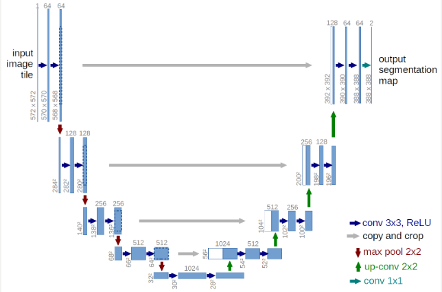
バイオメディカルのセグメンテーションのためのモデルのようです。
モデルの作成と学習・評価
ネットワークオブジェクトを定義して、学習を行っていきます。
model = network_unet()
model.compile(loss='binary_crossentropy', optimizer='adam', metrics=['acc'])

training = model.fit(image_train, label_train, epochs=EPOCHS, batch_size=12,
               shuffle=True, validation_data=(image_test, label_test), verbose=1)
今回は、0と1(255を正規化した値)の2値分類に相当しますので、'binary_crossentropy'を選択しています。
計算の状況を確認します。accurasyとlossをグラフ化してみました。
def plot_history(history):
    plt.plot(history.history['acc'])
    plt.plot(history.history['val_acc'])
    plt.title('model accuracy')
    plt.xlabel('epoch')
    plt.ylabel('accuracy')
    plt.legend(['acc', 'val_acc'], loc='lower right')
    plt.show()

    plt.plot(history.history['loss'])
    plt.plot(history.history['val_loss'])
    plt.title('model loss')
    plt.xlabel('epoch')
    plt.ylabel('loss')
    plt.legend(['loss', 'val_loss'], loc='lower right')
    plt.show()

plot_history(training)
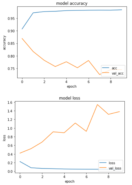
少しオーバーフィッティング気味かなという印象を受けます。
何はともあれ、出力画像が分割できているか確認してみましょう。
results = model.predict(image_train, verbose=1)

n = 20
plt.figure(figsize=(40, 4))
for i in range(n):
   ax = plt.subplot(3, n, i+1)
   plt.imshow(image_test[i].reshape(IMAGE_SIZE, IMAGE_SIZE))
   plt.gray()
   ax.get_xaxis().set_visible(False)
   ax.get_yaxis().set_visible(False)

   ax = plt.subplot(3, n, i+1+n)
   plt.imshow(results[i].reshape(IMAGE_SIZE, IMAGE_SIZE))
   plt.gray()
   ax.get_xaxis().set_visible(False)
   ax.get_yaxis().set_visible(False)

   ax = plt.subplot(3, n, i+1+2*n)
   plt.imshow(label_test[i].reshape(IMAGE_SIZE, IMAGE_SIZE))
   plt.gray()
   ax.get_xaxis().set_visible(False)
   ax.get_yaxis().set_visible(False)

plt.show()
原画像と分割画像と正解のラベル画像を並べてみました。

これままだまだ改良の余地がありそうですね。
おそらく前処理のどこかに問題があるか、255×255ピクセルの画像を64×64に圧縮しているのが悪いかは不明です。
また、違う結果がでたら報告できればと思います。
ではでは。
